
OpenCV is an instrumental library in real-time computer vision. Aside from its image processing functions, it is also open-source and free to use – a perfect partner for a board like Raspberry Pi. In this tutorial, you will learn how to install, operate, and create OpenCV projects using the Raspberry Pi. We will tackle all the fundamental functions and methods to work confidently with its framework.
Introduction
Computer Vision is a field (commonly placed under Artificial Intelligence) that trains computers to see and understand digital images. The area seeks to replicate tasks the human visual system does, including object detection, tracking, and recognition. These are easily implemented using OpenCV. And while OpenCV works better with more powerful systems than the Raspberry Pi, a credit-card sized computer, the Pi remains the first choice in DIY embedded solutions.
Installing OpenCV
There are two ways you can install OpenCV to the Raspberry Pi. First, using pip. Another is by manually building OpenCV from the source.
First Method
For a simple and fast solution, you can use pip to install OpenCV. Simply enter the following to the terminal.
pip install opencv-pythonor
pip install opencv-contrib-pythonNote that opencv-python and opencv-python-contrib are both unofficial pre-built binaries of OpenCV. This means some modules will not be available compared to when OpenCV is built from the source. Also, opencv-python only contains the OpenCV library’s main modules while opencv-python-contrib includes both main and contrib modules. If you’re saving space and don’t need additional functionalities that came with the contrib package, I suggest installing the first option. Otherwise, install opencv-python-contrib.
This whole process will take less than 5 seconds on a Raspberry Pi 4.
Second Method
For a more efficient installation, you can manually build OpenCV from the official source. This method is far from the one-liner code in the first method. This will take almost 3 hours to implement but will make the library more tailored to the Raspberry Pi, making it significantly faster to run.
Install the Dependencies
1. Like any other installations, update your Raspberry Pi first.
sudo apt update
sudo apt upgrade
2. Next, install OpenCV’s dependencies. There are a lot of them so we will install them in chunks so we can monitor what gets installed and what throws an error. The first chunk are packages we need to compile OpenCV.
sudo apt install cmake build-essential pkg-config git3. Next are packages that will add support for different image and video formats to OpenCV.
sudo apt install libjpeg-dev libtiff-dev libjasper-dev libpng-dev libwebp-dev libopenexr-dev
sudo apt install libavcodec-dev libavformat-dev libswscale-dev libv4l-dev libxvidcore-dev libx264-dev libdc1394-22-dev libgstreamer-plugins-base1.0-dev libgstreamer1.0-dev
4. Then, the packages that the OpenCV interface needs.
sudo apt install libgtk-3-dev libqtgui4 libqtwebkit4 libqt4-test python3-pyqt55. Next packages are crucial for OpenCV to run at a decent speed on the Raspberry Pi.
sudo apt install libatlas-base-dev liblapacke-dev gfortran6. Then, packages related to the Hierarchical Data Format (HDF5) that OpenCV uses to manage data.
sudo apt install libhdf5-dev libhdf5-1037. Lastly, the python-related packages.
sudo apt install python3-dev python3-pip python3-numpyUpsizing the Swap Space
The swap space is a portion of a computer’s main memory used by the operating system when the device runs out of physical RAM. It is a lot slower than RAM but we need it to help the process of compiling OpenCV to the Raspberry Pi. Enter the following command to access the swap file – the file that configures the swap space.
sudo nano /etc/dphys-swapfile2. Now replace the line
CONF_SWAPSIZE=100with
CONF_SWAPSIZE=2048Save and exit.
3. Lastly, restart the service on your Raspberry Pi to implement the changes without rebooting the system.
sudo systemctl restart dphys-swapfileCongratulations, you now changed your swap space from 100MB to 2GB.
Cloning the OpenCV Repositories
At last, we are now ready to get the actual OpenCV files. Enter the following commands to clone the OpenCV repositories from GitHub to your computer. Hopefully, your present working directory is your home directory. It’s not required, but I suggest cloning it there, so it’s easily accessible. These files are also large, so depending on your internet connection, this may take a while.
git clone https://github.com/opencv/opencv.git
git clone https://github.com/opencv/opencv_contrib.git
Compiling OpenCV
1. You can see both repositories on your home directory after you successfully cloned them. Now, let’s create a subdirectory called “build” inside the OpenCV folder to contain our compilation.
mkdir ~/opencv/build
cd ~/opencv/build
2. Next, generate the makefile to prepare for compilation. Enter the following command:
cmake -D CMAKE_BUILD_TYPE=RELEASE -D CMAKE_INSTALL_PREFIX=/usr/local -D OPENCV_EXTRA_MODULES_PATH=~/opencv_contrib/modules -D ENABLE_NEON=ON -D ENABLE_VFPV3=ON -D BUILD_TESTS=OFF -D INSTALL_PYTHON_EXAMPLES=OFF -D OPENCV_ENABLE_NONFREE=ON -D CMAKE_SHARED_LINKER_FLAGS=-latomic -D BUILD_EXAMPLES=OFF..3. Once the make file is done, we can now proceed to compile. The argument j$(nproc) tells the compiler to run using the available processors. So for example, nproc is 4, it will be -j4. This will take the longest time out of all the steps. For reference, a newly set up Raspberry Pi 4 with 8GB RAM takes more than an hour to execute this command.
make -j$(nproc)4. Hopefully, the compilation didn’t take more than 2 hours of your life. We now proceed to install the compiled OpenCV software.
sudo make install5. Finally, we regenerate the Pi’s library link cache. The Raspberry Pi won’t be able to find OpenCV without this step.
sudo ldconfigReverting the Swap Space
1. Now that we are done installing OpenCV, we don’t need to have such a large swap space anymore. Access the swap space again with the following command.
sudo nano /etc/dphys-swapfile2. Change the line
CONF_SWAPSIZE=2048to
CONF_SWAPSIZE=100Save and Exit.
3. Lastly, restart the service to implement the changes.
sudo systemctl restart dphys-swapfileTesting
1. The easiest way to confirm our installation is by bringing up an interactive shell and try to import cv2 (OpenCV’s library name). Open python.
python2. Now, it doesn’t matter what version you are using, if you followed the steps before, OpenCV should already be accessible in both Python 2 and Python 3. Try to import it using the line:
import cv23. If the import line returned nothing, then congratulations! Additionally, you can verify the OpenCV version you have in you computer using the following command:
cv2.__version__Now that we have OpenCV in our Raspberry Pi, let us proceed with learning how to use its essential functions.
Image Input
Firstly, we need input. Image processing needs an image to work on, after all. There are 3 types of image input: Still image, Video, and Video Stream.
Still Image
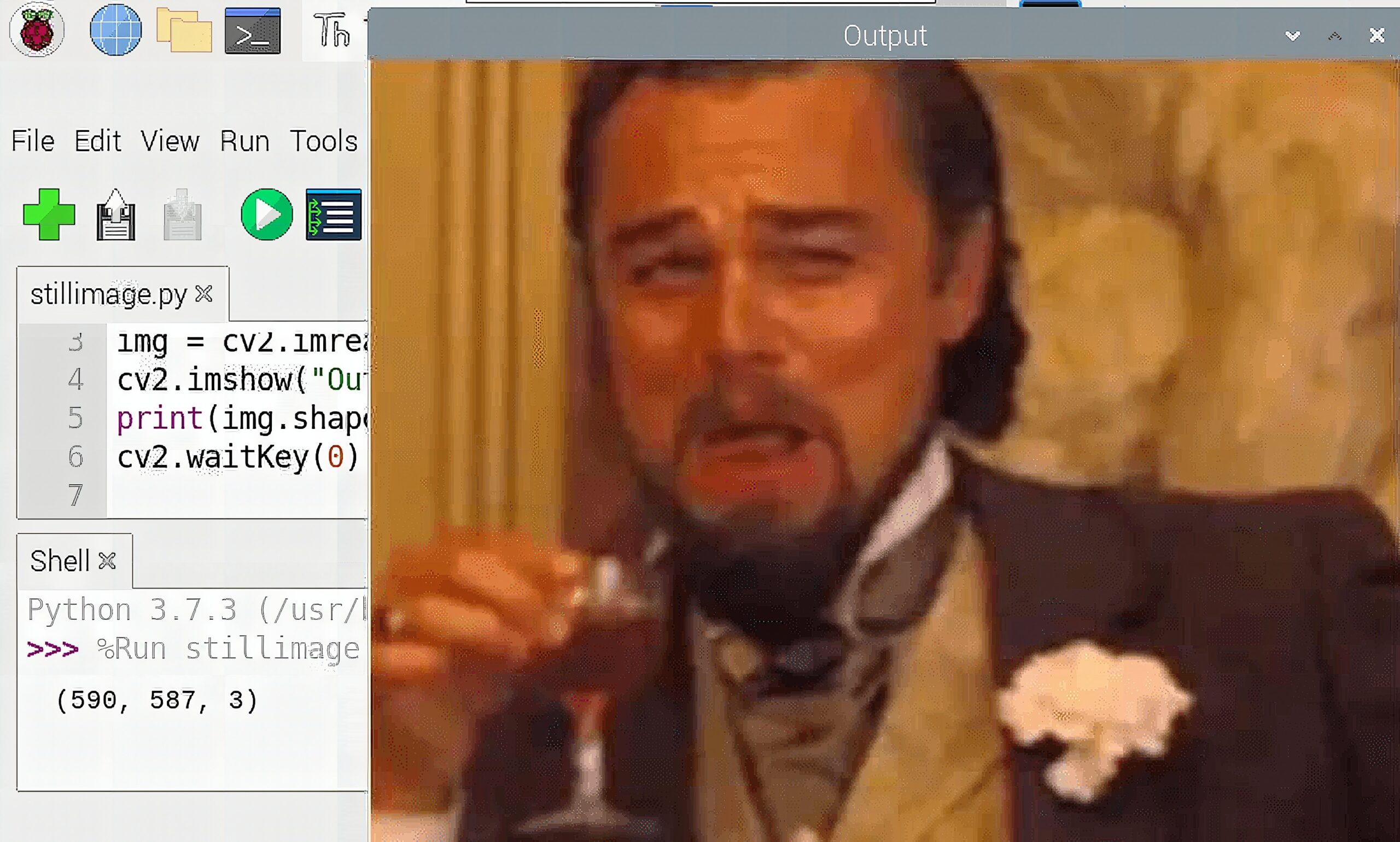
To use a still image, we use the imread function. It simply loads an image from a specified file path and returns it. If the image cannot be read, it will return an empty matrix.
Furthermore, to show the image, we use the imshow function. It displays the image in a window which automatically fits with the image size. The first argument of the function is the window name, while the second argument is the image source, which is the variable img.
We also need the waitKey function to display the image indefinitely. It has an argument of time in milliseconds. If the value is 0, it will wait until a keyboard button is pressed. If you press a key while waitKey is active, your program continues to the next lines.
import cv2 img = cv2.imread("Resources/picture.png")
cv2.imshow("Output",img)
cv2.waitKey(0)
Video
For video, we first use the VideoCapture function to create a video object. Its argument is the device index, the pathname to a video file, or the streaming URL of your camera. A device index is a number that specifies the camera device in your system. For instance, you write 0 to use the built-in webcam on your laptop. If you’re using an IP camera that streams to a specific IP address in your home network, you can use VideoCapture to get that stream to OpenCV. Just write the URL of the camera instead of a device index or a video file path.
After creating a video object, you can then read the frames from it using read(). It also returns a boolean that tells you True if the frame is read correctly or False if not.
Similarly to still images, we use imshow and waitKey to display the video output. However, you need to tweak the time argument on the waitKey function to play the video in its native framerate. For instance, if the video is 30 frames per second. You must convert it first to milliseconds by dividing 30 by 1000. The following line 0XFF ==ord('q') makes the code stop if the q key is pressed.
import cv2 cap = cv2.VideoCapture("Resources/video.mp4")
while True: success, img = cap.read() cv2.imshow("Video", img) if cv2.waitKey(30) & 0XFF ==ord('q'): break
Camera Stream
Meanwhile, with video streams, you need to replace the video file’s pathname with your camera device’s index. Additionally, you can set the dimensions of the video using the set function. The waitKey argument can be set to any value depending on your preference.
import cv2 cap = cv2.VideoCapture(0)
cap.set(3,640)
cap.set(4,480) while True: success, img = cap.read() cv2.imshow("Video", img) if cv2.waitKey(1) & 0XFF ==ord('q'): break
The cv2.VideoCapture() function works only for USB cameras, not for CSI cameras. That is why if you want to use the Raspberry Pi camera, you need to import an additional Python library called picamera.
To install picamera simply enter the following in the terminal:
sudo pip install picameraThe code is pretty similar with the previous examples. It just slightly differs with some notations and labels. See the code below.
from picamera.array import PiRGBArray
from picamera import PiCamera
import cv2 camera = PiCamera()
camera.resolution = (320, 240)
camera.framerate = 30
camera.brightness = 65 raw_capture = PiRGBArray(camera, size=(320,240)) for frame in camera.capture_continuous(raw_capture, format="bgr", use_video_port=True): img = frame.array cv2.imshow("Original Image", img) raw_capture.truncate(0) if cv2.waitKey(1) & 0xFF==ord('q'): break
Now that we have the image input, we can now use OpenCV’s magic for image processing.
Basic Methods and Functions
It’s debatable what functions are to be considered as basic and essential to OpenCV’s framework. I chose the following functions based on the tutorials I read and watched over the past few weeks. These functions are commonly used for pre-processing images for computer vision.
Grayscale
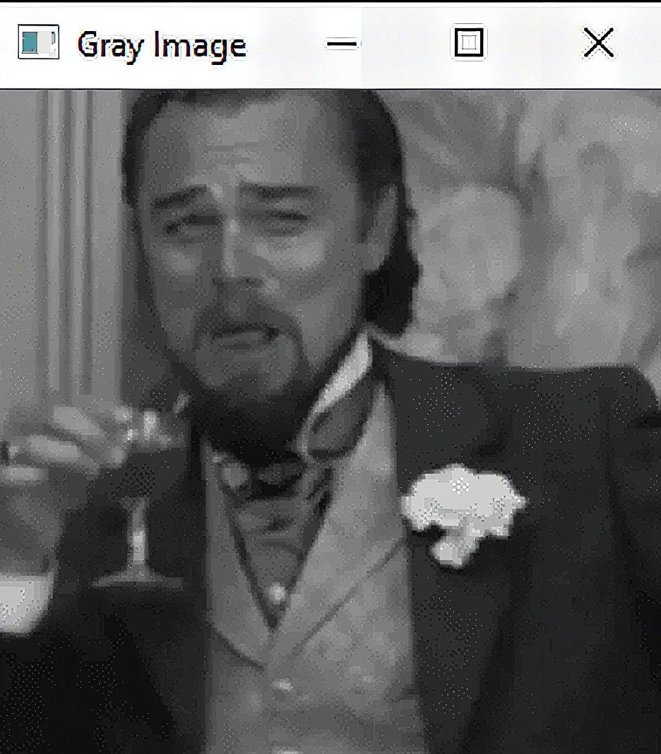
First, <a href="Color Space Conversions">cvtColor</a>. It converts an image from one color space to another. Note that the default color format in OpenCV is BGR (the bytes are reversed compared to standard RGB). We often use this method to convert images to Grayscale or HSL for pre-processing. It requires at least 2 parameters, which are the image src and the color space conversion code. In our example, we use the code COLOR_BGR2GRAY to convert the image to grayscale as a prep for edge detection.
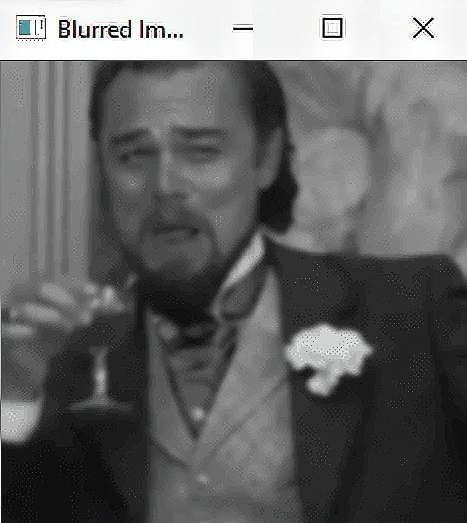
Gaussian Blur
Next is <a href="Image Filtering">GaussianBlur</a>. This function blurs an input image using a Gaussian filter. It requires at least 3 parameters: img src, kernel size, and sigmaX. The kernel size must always be positive and odd. The kernel standard deviation in the x direction sigmaX, also determines sigmaY if only sigmaX is defined. If both are given as zeros, they are calculated from the kernel size. This function is commonly used in removing Gaussian noise from an image and image smoothening.
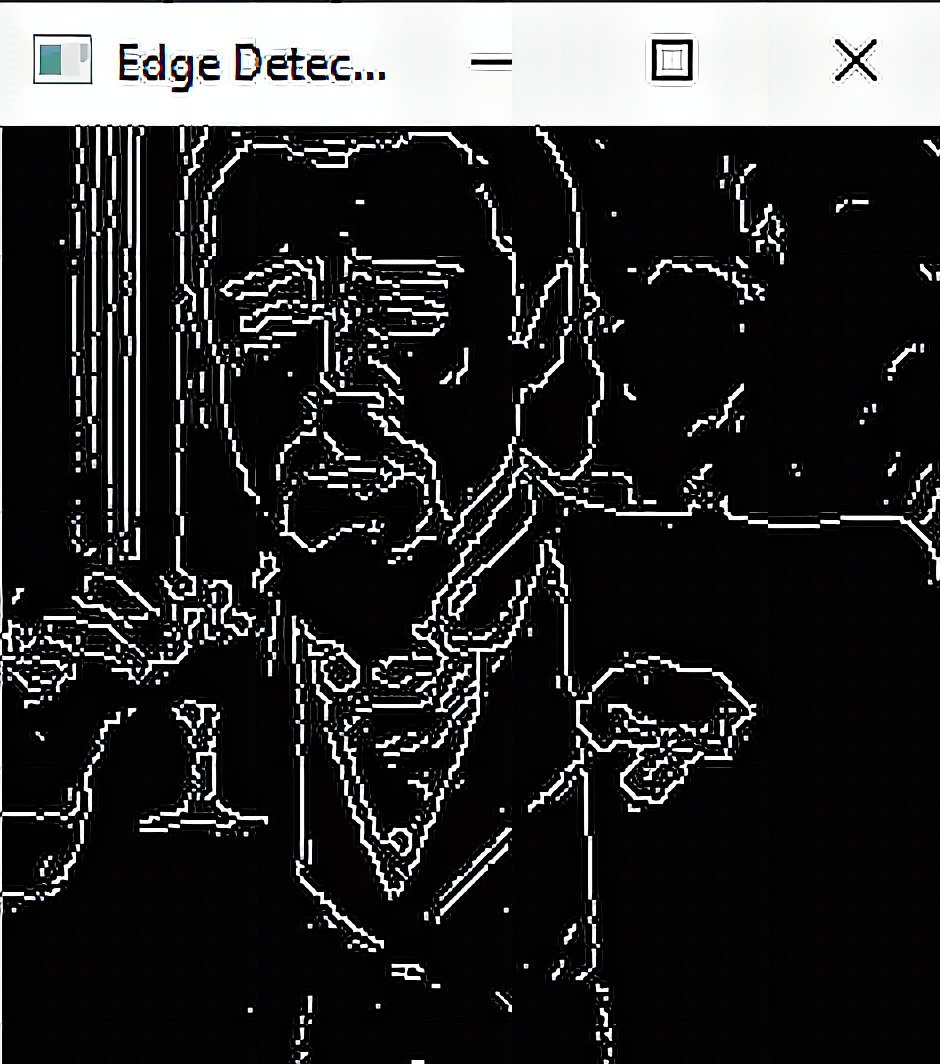
Canny Edge Detection
Third is the <a href="Feature Detection">Canny</a> function. It finds edges in an input image using Canny algorithm. It requires at least 3 parameters: img src, minVal, and maxVal. minVal is used for edge linking while maxVal is used to find initial segments of strong edges.
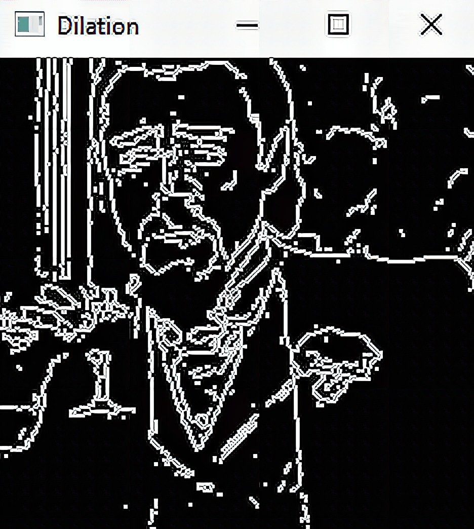
Dilate
Penultimate one is dilate. It exaggerates the features of an image using a specific structuring element. It requires at least 3 parameters: image src, kernel, and iteration number. The kernel is the structuring element for dilation. On the sample code, we use numpy to create a 5×5 matrix of ones as a kernel for dilate. The iteration number is the number of times dilation is applied.
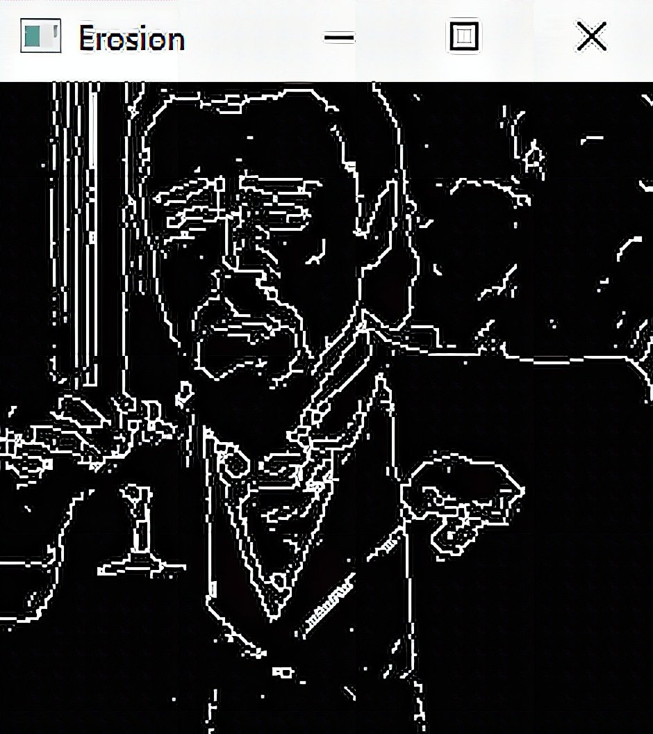
Erode
Last is the sister function of dilate, erode. It chisels or cuts down the image using a specific structuring element. It also requires at least 3 parameters: image src, kernel, and iteration number. We use the same kernel from dilate to cut down and reveal the individual elements and joining disparate elements in an image. Both dilate and erode works as a pair to remove noise and isolate intensity bumps or holes in an image.
import cv2
import numpy as np img = cv2.imread("Resources/picture.png")
kernel = np.ones((5,5), np.uint8) imgGray = cv2.cvtColor(img, cv2.COLOR_BGR2GRAY)
imgBlur = cv2.GaussianBlur(imgGray, (11,11), 0)
imgCanny = cv2.Canny(img, 120, 120)
imgDilate = cv2.dilate(imgCanny, kernel, iterations=1)
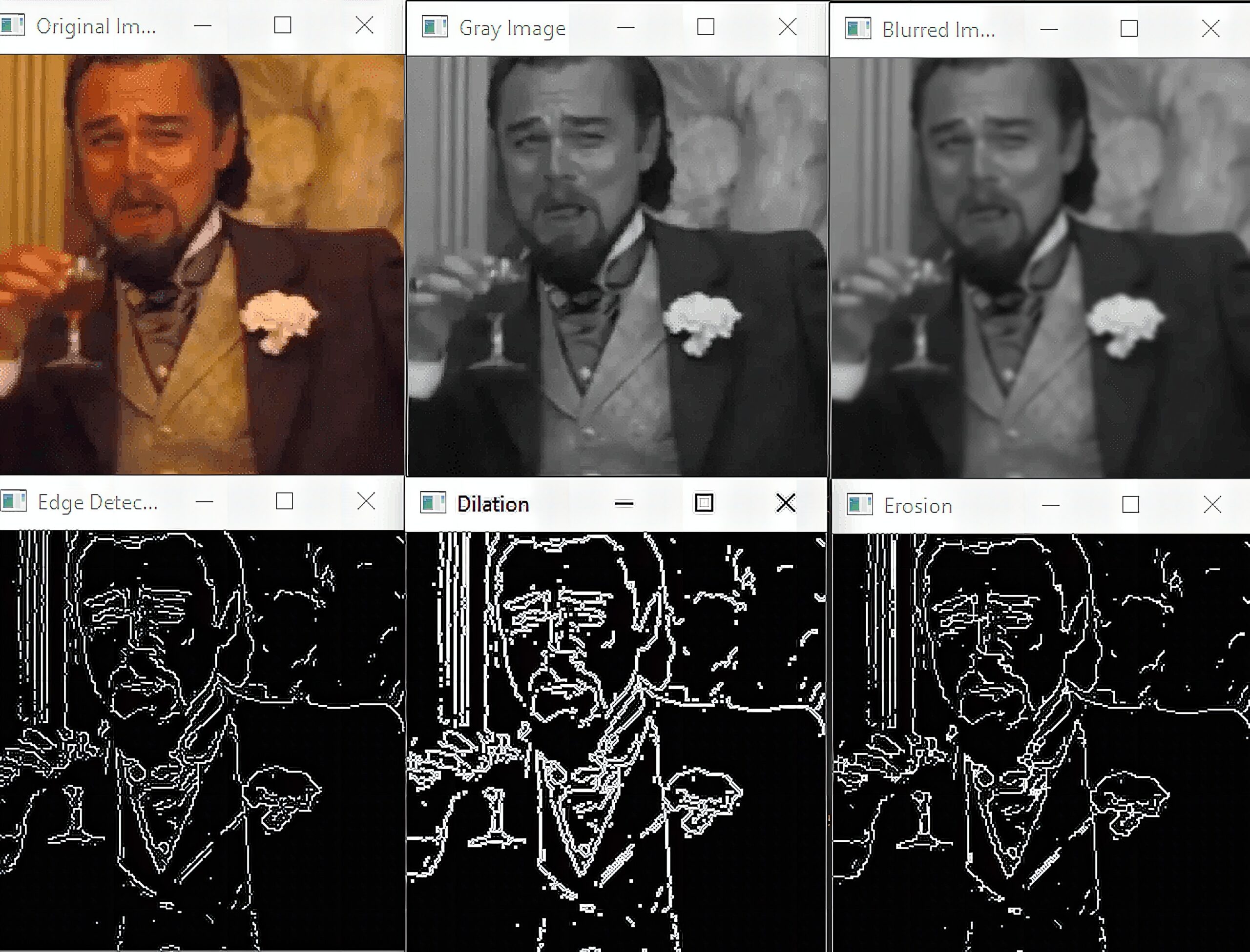
imgErode = cv2.erode(imgDilate, kernel, iterations=1) cv2.imshow("Original Image", img)
cv2.imshow("Gray Image", imgGray)
cv2.imshow("Blurred Image", imgBlur)
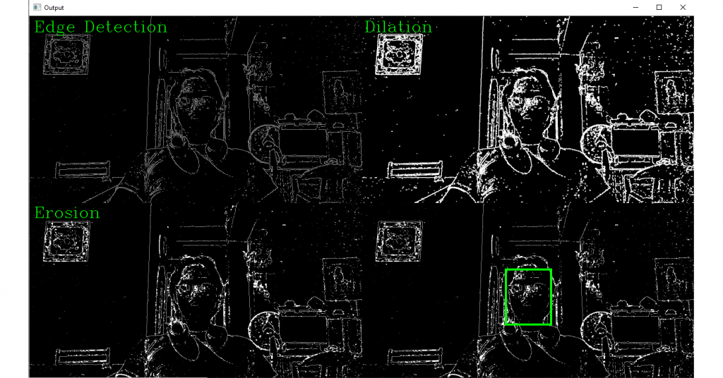
cv2.imshow("Edge Detection", imgCanny)
cv2.imshow("Image Dilation", imgDilate)
cv2.imshow("Image Erosion", imgErode) cv2.waitKey(0)Crop and Resize
In OpenCV, the convention for images is that (0,0) is in the top left most corner of a photo. Given point A(100, 140), it would be 100 pixels to the left and 140 pixels downward. Now to confuse us even further, to crop an image, you indicate 2 ranges, y first then x. For instance if we want to crop variable img from the 200th to the 300th x pixel and 0 to the 100th y pixel, we must write img[0:100,200:300].
Thankfully, resizing isn’t a problem anymore as we can always use resize(). It only requires 2 parameters: image src and target size. If the target dimensions aren’t proportional to your image’s actual dimensions, your output image will be deformed.
import cv2
import numpy as np img = cv2.imread("Resources/picture.png")
print(img.shape)
imgResize = cv2.resize(img, (300,300))
imgCrop = imgResize[0:100,200:300]
cv2.imshow("Output", img)
cv2.imshow("Resized Output", imgResize)
cv2.imshow("Cropped Output", imgCrop)
cv2.waitKey(0)
Shapes and Texts
You need to learn how to create shapes and texts to emphasize the objects you detect in your image. It’s one thing to detect faces and objects, creating a bounding rectangle for your detections is another.
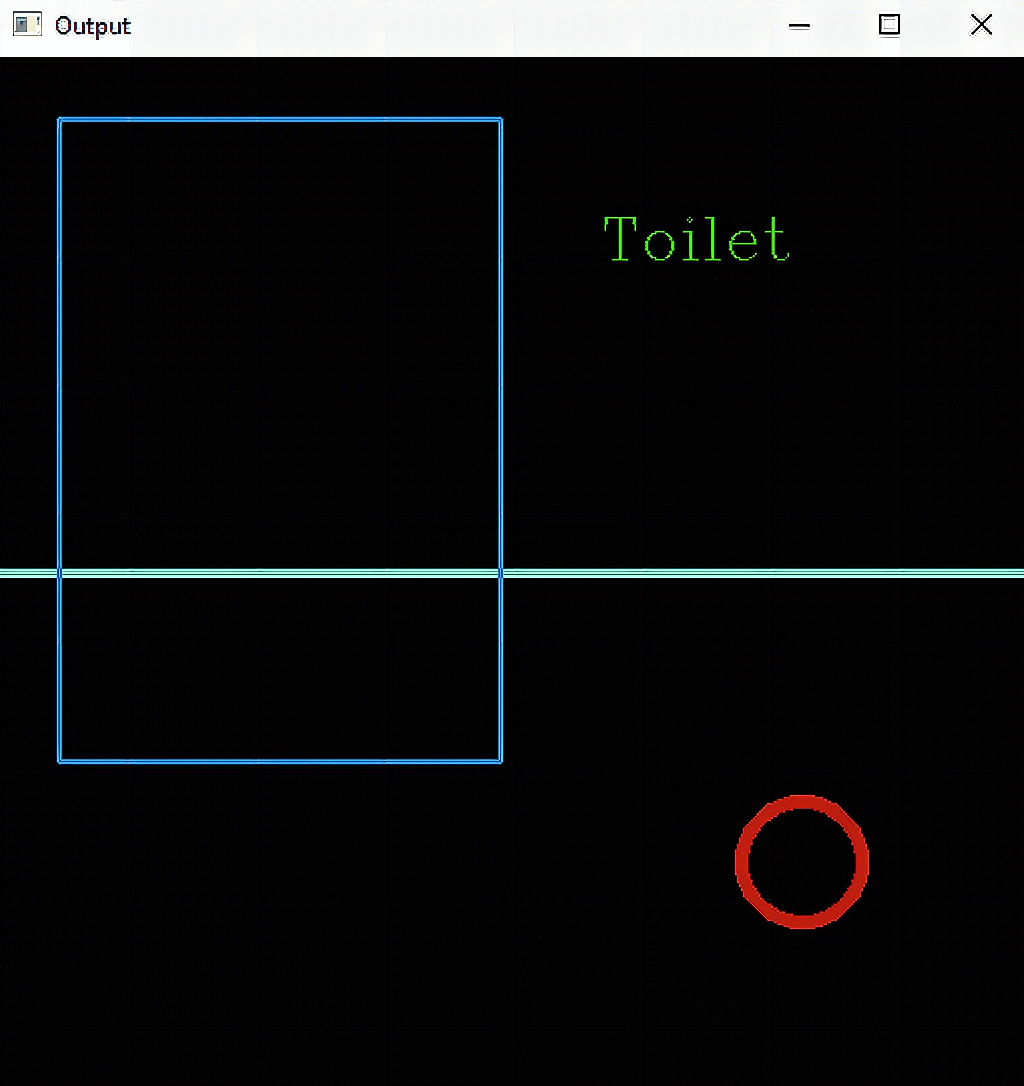
For our example, we will not use imread to load an image. Instead, we will create a blank canvas using a NumPy function called zeros. This will create 3 channels with a 512 x 512 array filled with zeros. We then set the maximum value of the elements in the array to 255 using uint8 to emulate a standard RGB/BGR image. Since all the values are zeros, the image will be a black square.
Line
Now we draw a line using <a href="Drawing Functions">line()</a>. You need to enter at least 5 parameters: the image src, the starting and ending coordinates, the color in BGR, and the thickness. In our example, we cut the square horizontally in half by a starting point of (0,256) and ending point of (512,256). The color values, which I entered arbitrarily, produced light blue while the thickness is 2.
Rectangle
Next is <a href="Drawing Functions">rectangle()</a>. To draw a rectangle, you also need at least 5 parameters: image src, the top left, the bottom right coordinates, the color, and the thickness. All works the same with line.
Circle
Third is <a href="Drawing Functions">circle()</a>. You need at least 5 parameters for this function: image src, the center of the circle, the radius, the color, and the thickness. Additionally, you can create a filled circle by entering a negative thickness value.
Text
Finally we write text using putText() function. To write a specified text, you need to enter at least 7 parameters: image src, text string, the bottom left starting coordinate of the text, the font face, the scale, the color, and the scale. The font face is the font type. The available styles are in this link. Moreover, the scale is just a factor that is multiplied by the font-specific base size.
import cv2
import numpy as np img = np.zeros((512,512,3),np.uint8) cv2.line(img,(0,256),(512,256),(200,232,132),3)
cv2.rectangle(img, (0,0),(250,350),(213,123,23),2)
cv2.circle(img,(400,50),30,(14,29,195),5)
cv2.putText(img, "Toilet", (300,100), cv2.FONT_HERSHEY_COMPLEX,3,(0,213,51),1) cv2.imshow("Output", img)
cv2.waitKey(0)
Now that we have shape and text creating under our belt, we can proceed on more advanced functionalities like warp perspective.
Warp Perspective

Warp perspective lets you change the perspective on your images. For example, you have a piece of paper captured in your video. This function enables you to have a bird’s eye view of that piece of paper to read it better, especially when paired with other image processing techniques. We usually use this for document scanning and optical mark recognition.
Warp perspective does not change the image content but deforms the pixel grid and maps this deformed grid to the destination image. To do that, you need 2 sets of four pairs of points. The first set determines the corners of the object in the source image, while the second set determines the points of the corresponding quadrangle vertices in the destination image. Since we want the corners of the object to lay on the edges of the new image, we use the second image’s extreme coordinates, such as [0,0] and [width, height].
After we set the 2 arrays, we use getPerspectiveTransform() to retrieve a matrix map of the transformed image. Then, use warpPerspective() to implement the matrix to the source image.
import cv2
import numpy as np img = cv2.imread("Resources/box.jpg")
width, height = 500, 300 points1 = np.float32([[109,155],[714,51],[75,560],[890,424]])
points2 = np.float32([[0,0],[width,0],[0,height],[width,height]])
matrix = cv2.getPerspectiveTransform(points1,points2)
imgOutput = cv2.warpPerspective(img, matrix, (width, height))
cv2.imshow("Original", img)
cv2.imshow("Output", imgOutput)
cv2.waitKey(0)
In our example, we set the corners manually by indicating the coordinates in an array. But we can also use another function to detect the corners automatically. We will discuss this in a later part of the article.
Color Detection
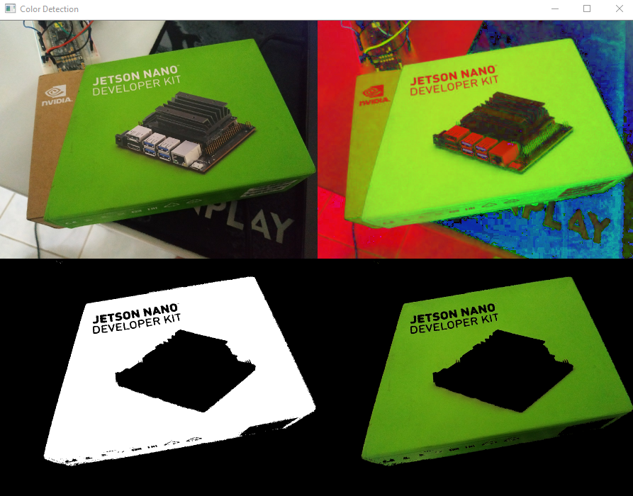
Color detection is the process of detecting a specific color in an image. This may be herculean of a task with other frameworks, but it is pretty simple with OpenCV – you just need track bars and a good set of eyes.
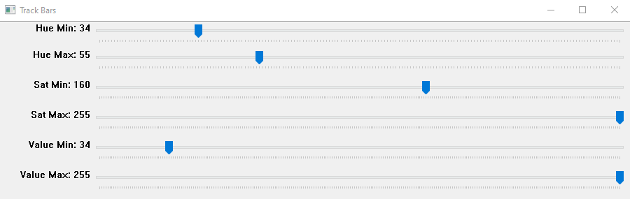
First, we create a window using namedWindow() to house all of our trackbars. We then resize it using resizeWindow() depending on the number of trackbars we will add, in our case, 6.
Next, we create the trackbars using createTrackbar(). You need at least 5 parameters: the trackbar name, the specified window, the initial value, the maximum value, and a function that activates when the slider is used. The initial value is an integer, which reflects the position of the slide upon creation. Unfortunately, the function is required even if you don’t need your slider to activate anything. Hence, we create an empty function that does nothing besides fulfilling this odd requirement.
For the main loop, we endlessly read the target image using imread(), convert it to HSV using cvtColor(), and update the trackbar positions using getTrackbarPos().
HSV (hue, saturation, value) colorspace is an alternative model of RGB. Since the hue channel models the color type, it is instrumental in color filtering and detection. Meanwhile, saturation goes from unsaturated to represent shades of gray and fully saturated (no white component). The value channel defines the intensity or brightness of the color. We associate the corresponding HSV values to a track bar of its own, namely Hue Minimum and Maximum, Saturation Minimum and Maximum, and Value Minimum and Maximum.
Next, we use inRange() to check if the current trackbar positions lie between the elements of lower and upper boundaries. This will create an image wherein white represents the values between the lower and upper boundaries and black otherwise – extracting the region of interest. We then use bitwise_and() to exclude all values in the image except the ones inside the region of interest.
import cv2
import numpy as np def empty(a): pass path = "Resources/box.jpg" cv2.namedWindow("Track Bars")
cv2.resizeWindow("Track Bars",(640,240))
cv2.createTrackbar("Hue Min", "Track Bars", 34, 179, empty)
cv2.createTrackbar("Hue Max", "Track Bars", 55, 179, empty)
cv2.createTrackbar("Sat Min", "Track Bars", 160, 255, empty)
cv2.createTrackbar("Sat Max", "Track Bars", 255, 255, empty)
cv2.createTrackbar("Value Min", "Track Bars", 34, 255, empty)
cv2.createTrackbar("Value Max", "Track Bars", 255, 255, empty) while True: img = cv2.imread(path) imgHSV = cv2.cvtColor(img,cv2.COLOR_BGR2HSV) hmin = cv2.getTrackbarPos("Hue Min","Track Bars") hmax = cv2.getTrackbarPos("Hue Max", "Track Bars") smin = cv2.getTrackbarPos("Sat Min", "Track Bars") smax = cv2.getTrackbarPos("Sat Max", "Track Bars") vmin = cv2.getTrackbarPos("Value Min", "Track Bars") vmax = cv2.getTrackbarPos("Value Max", "Track Bars") lower = np.array([hmin,smin,vmin]) upper = np.array([hmax,smax,vmax]) mask = cv2.inRange(imgHSV,lower,upper) imgResult = cv2.bitwise_and(img,img,mask=mask) cv2.imshow("Original Image", img) cv2.imshow("HSV Image", imgHSV) cv2.imshow("Mask", mask) cv2.imshow("Final Output", imgResult) cv2.waitKey(1)
Contour Detection
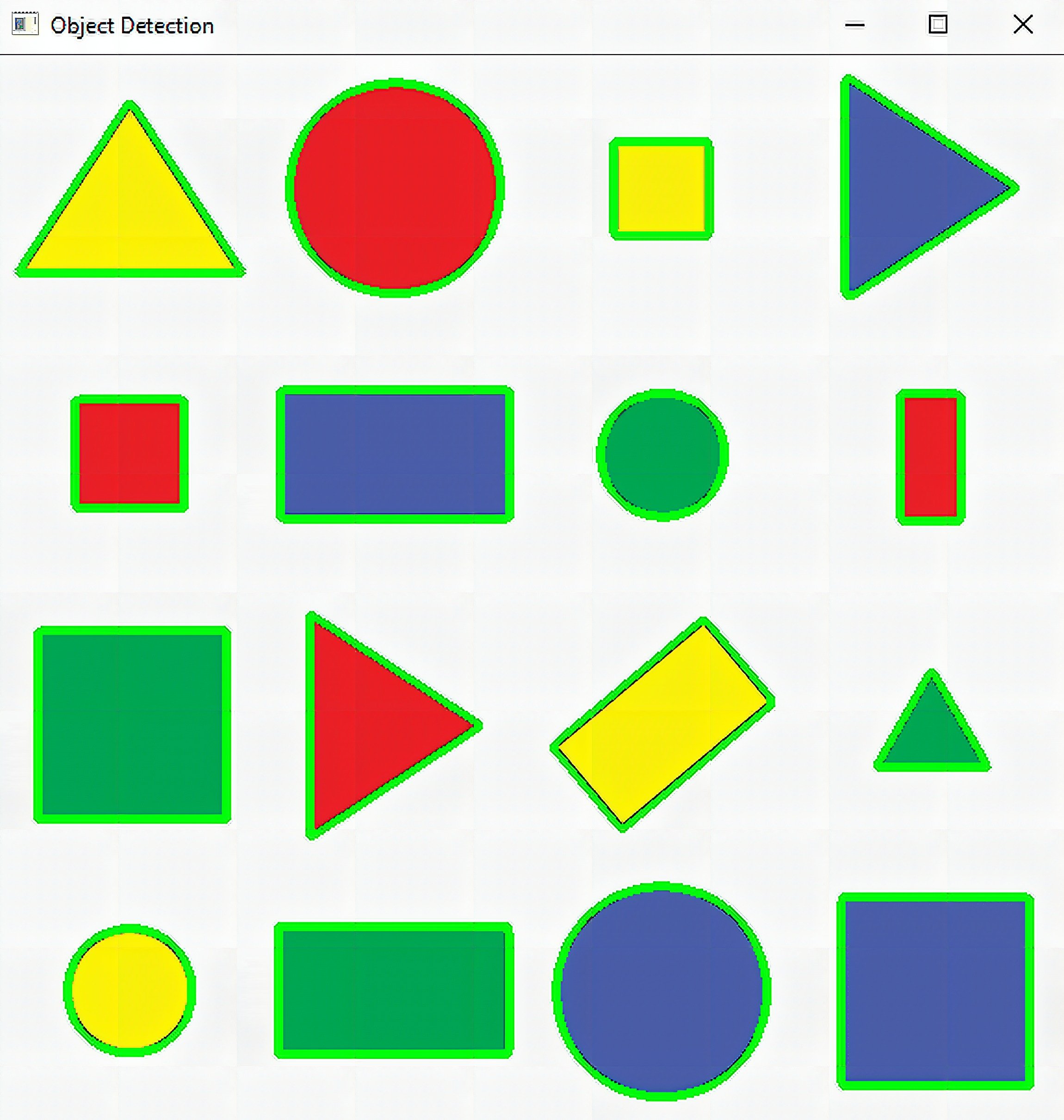
Contour detection is the process of joining all the continuous points along an object’s boundary. Contours are necessary for object detection, recognition, and shape analysis.
We start by duplicating our original image using the method copy. This way, we draw the contours on a separate image rather than writing on the actual image itself. Next, we proceed with the pre-processing. First, convert it to Grayscale to ease up edge detection. Then, we use Gaussian blur to smooth out the edges. Finally, use Canny to detect the edges.
Now that we have a binary image courtesy of Canny, we use it as an input to findContours(), which retrieves contours from binary images. Contours are the raw shapes that enclose the objects detected in your image. This function requires at least 3 parameters: image src, mode, and method. The contour retrieval mode defines the contour retrieval algorithm. We specifically use RETR_EXTERNAL because it retrieves only the extreme outer contours. See all retrieval modes here. On the other hand, the method defines the contour approximation algorithm. The CHAIN_APPROX_NONE method that we used stores absolutely all the contour points, creating an enclosing shape on the object. For reference, there’s also the CHAIN_APPROX_SIMPLE method that stores only the corners of the object.
We now use a loop to validate the detected contours and draw on them. For every detected contour, we get the area using contourArea(). If the area is larger than an explicit number (change this according to your image size), then the contour is valid. We now draw on it using drawContours(). This function requires at least 5 parameters: the image src, the particular contour, the contour index, color, and thickness. The index of the contour indicates the contour to be drawn. If it is -1, all the contours are drawn.
Other additional functions commonly associated with contours are arcLength() and approxPolyDP(). You can use them to obtain the perimeter and the number of corners of the object, respectively.
import cv2
import numpy as np path = "Resources/shapes.png"
img = cv2.imread(path) imgContour = img.copy() imgGray = cv2.cvtColor(img,cv2.COLOR_BGR2GRAY)
imgBlur = cv2.GaussianBlur(imgGray, (7,7), 1)
imgCanny = cv2.Canny(imgBlur,100,100) contours, hierarchy = cv2.findContours(imgCanny,cv2.RETR_EXTERNAL,cv2.CHAIN_APPROX_NONE) for cnt in contours: area = cv2.contourArea(cnt) print("area: " + str(area)) if area>500: cv2.drawContours(imgContour, cnt, -1, (0, 255, 0), 3) para = cv2.arcLength(cnt,True) print("perimeter: " + str(para)) approx = cv2.approxPolyDP(cnt,0.02*para,True) print("approximate points: " + str(len(approx))) cv2.imshow("Contour Detection",imgContour)
cv2.waitKey(0)
Object Detection using Cascades
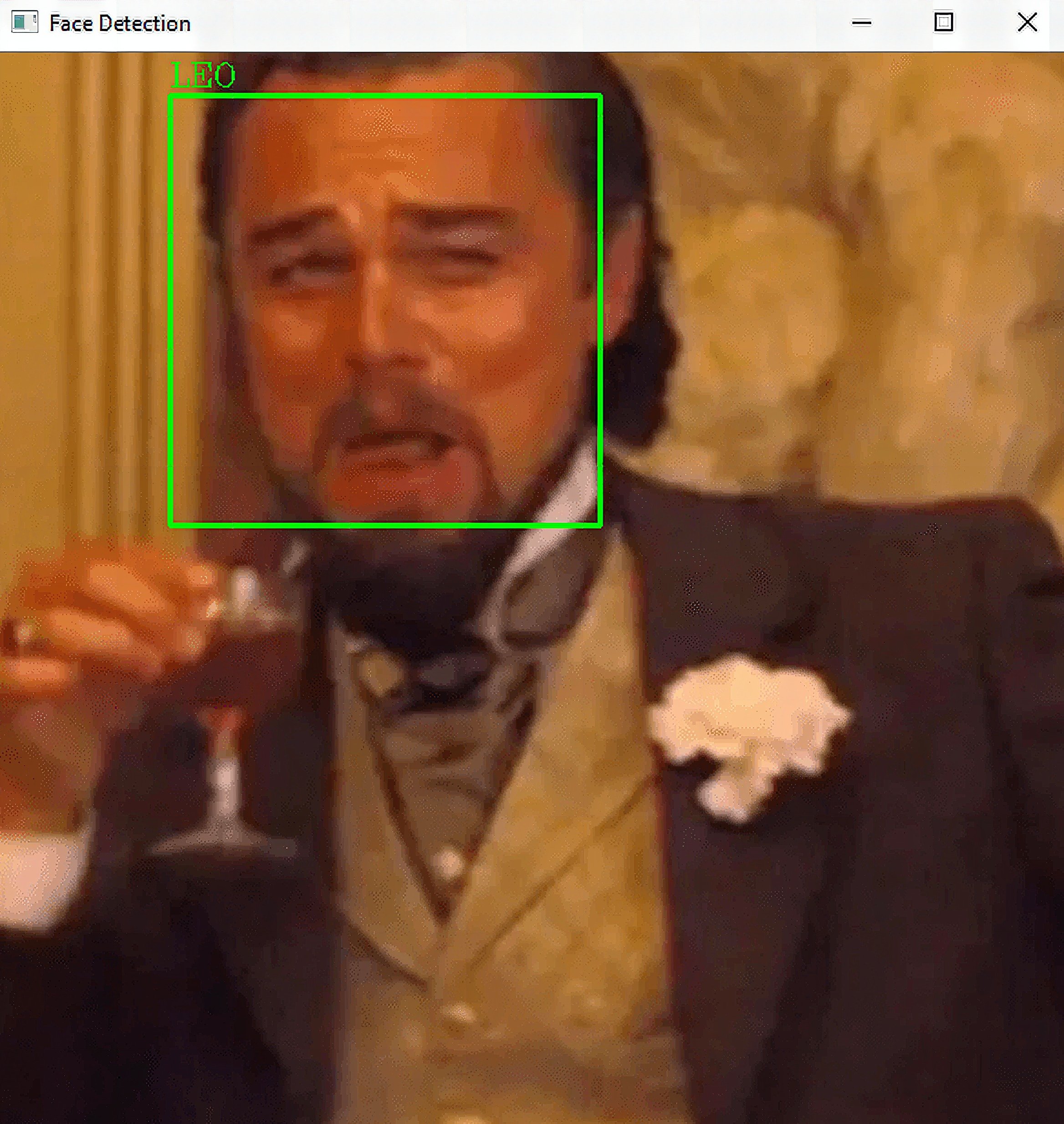
For our finale, we will use a haar cascade to detect a face in an input image. This must sound daunting at first, but take a peek at the code and see how short it is. This is the magic of machine learning.
Haar Cascade is a machine learning object detection algorithm used to identify faces and objects in an image based on the concept proposed by Paul Viola and Michael Jones in 2001. Since then, Haar Cascades have been widely used in many academic papers and computer vision applications, including OpenCV. Don’t worry; we don’t need to know how the intricacies of the model work. We just need to know how to use it with OpenCV.
First, download the haar cascade optimized for frontal face detection on OpenCV’s GitHub page. Load it using CascadeClassifier(). Then prep the image by converting it to grayscale. Next, we use detectMultiScale() to detect objects of different sizes within the input image. The detected objects are returned as a list of bounding rectangles. This function needs 3 parameters: image src, scale factor, and the number of minimum neighbors. The scale factor defines how much the image size is reduced at each image scale, while the number of minimum neighbors indicates how many neighbors each candidate rectangle should have to retain it. You can tweak both these parameters to adjust the sensitivity of the object detection algorithm.
After detecting the faces, just like the contour example, we use a loop to draw rectangles and labels on it.
import cv2 faceCascade = cv2.CascadeClassifier("Resources/haarcascade_frontalface_default.xml") img = cv2.imread("Resources/picture.png")
imgGray = cv2.cvtColor(img,cv2.COLOR_BGR2GRAY) faces = faceCascade.detectMultiScale(imgGray,1.1,39)
for (x,y,w,h) in faces: cv2.rectangle(img,(x,y),(x+w,y+h),(0,255,0),2) cv2.putText(img, "LEO",(x,y-5),cv2.FONT_HERSHEY_COMPLEX, 0.6, (0,255,0),1) cv2.imshow("Face Detection",img) cv2.waitKey(0)
As a bonus, here’s a code that uses your computer’s webcam to detect faces in real-time. I think almost all webcam software has this already, but it is still fun to know that you can code it yourself, and it actually works.
import cv2
import numpy as np cap = cv2.VideoCapture(0)
cap.set(3,640)
cap.set(4,480) faceCascade = cv2.CascadeClassifier("Resources/haarcascade_frontalface_default.xml")
while True: success, img = cap.read() imgGray = cv2.cvtColor(img,cv2.COLOR_BGR2GRAY) faces = faceCascade.detectMultiScale(imgGray,1.1,39) for (x,y,w,h) in faces: cv2.rectangle(img,(x,y),(x+w,y+h),(0,255,0),2) cv2.putText(img, "TOILET",(x,y-10),cv2.FONT_HERSHEY_COMPLEX, 0.6, (0,255,0),1) cv2.imshow("Output",img) if cv2.waitKey(1) & 0xFF==ord('q'): break
This was honestly longer than I anticipated. I initially wanted to write just for the Raspberry Pi, but it turned out a fully-fledged OpenCV article. If you managed to get down here, congrats! You now have a solid understanding of how OpenCV works. The thing is pretty impressive, really. I hope you learned as much I did. See you in the next article!
Frequently Asked Questions
[faq] [faq_q]Which Raspberry Pi version is best for OpenCV?[/faq_q] [faq_a]Raspberry Pi 4 with 4GB or 8GB RAM is the sweet spot. The Pi 3 works for lighter projects, the Pi 5 cuts inference times further. OpenCV runs on all of them, just at different speeds.[/faq_a][faq_q]Do I need to compile OpenCV from source on Raspberry Pi?[/faq_q] [faq_a]For most projects, no. Running pip install opencv-python works on recent Raspberry Pi OS versions. Compile from source only for custom CUDA support, specific build flags, or a particular OpenCV version not available via pip.[/faq_a][faq_q]Can I use the Raspberry Pi camera module with OpenCV?[/faq_q] [faq_a]Yes. Use picamera2 to capture frames, then pass the numpy array to OpenCV functions. On older OS versions, OpenCV VideoCapture(0) also works if the camera is set up as a V4L2 device.[/faq_a][faq_q]What is the difference between OpenCV and PyTorch for face detection?[/faq_q] [faq_a]OpenCV cv2.dnn runs pre-trained models for inference only and does not need PyTorch installed. PyTorch lets you train new models. For deploying face detection on Pi, OpenCV is faster and lighter.[/faq_a][faq_q]How fast is face detection on Raspberry Pi 4?[/faq_q] [faq_a]Around 5-15 FPS for Haar cascade or HOG-based methods. DNN-based methods like Yunet or RetinaFace typically run 2-8 FPS on Pi 4. Pi 5 is roughly 2x faster across all of these.[/faq_a][/faq]Frequently Asked Questions
What does this The Ultimate OpenCV with Raspberry Pi Tutorial tutorial cover?
OpenCV is an instrumental library in real-time computer vision.
Which Raspberry Pi model fits the The Ultimate OpenCV with Raspberry Pi Tutorial project?
Pi 4 (4GB) or Pi 5 for desktop apps and AI workloads. Pi Zero 2 W is enough for headless / sensor builds. Pi 3 B+ works but is slower for camera or ML.
How do I auto-start the The Ultimate OpenCV with Raspberry Pi Tutorial script on boot?
Use systemd. Create /etc/systemd/system/myproject.service with ExecStart=/usr/bin/python3 /home/pi/script.py and Restart=always. sudo systemctl enable myproject.