Neural Networks: Creating a Perceptron Model in Python

In this tutorial, you will learn the fundamentals of neural networks and deep learning – the intuition behind artificial neurons, the standard perceptron model, and the implementation of the model in Python. This will be an introductory article to a series of neural networks and deep learning tutorials. However, you need at least basic knowledge in Math and Python to grasp the articles’ ideas fully.

Biological Neurons

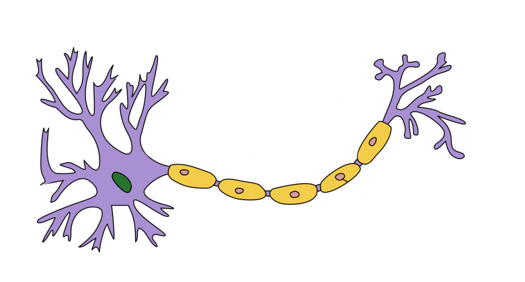
Neurons are interconnected nerve cells that process and transmits electrochemical signals in the brain. There are approximately 100 billion of them inside of us, with each neuron connected to about 10,000 other neurons.

A neuron starts working when a dendrite receives information (in the form of electrochemical energy) from other neurons. It modulates the signal then passes the information to the cell nucleus or soma (the green blob in Figure 1) for processing. Then, the Soma sends the output data through the axon (the yellow bridge) to the Axon output terminals or Synapse. The Synapses send the data to the next neurons.

Each neuron consists of multiple dendrites which means there are multiple inputs as well. If the sum of these electrical inputs exceeds a certain threshold, the Soma will activate the neuron, passing the signal to other neurons which may then trigger again.

Note that neurons only activate if the total signal received exceeds a certain threshold. It’s either no, we will not send a signal, or yes, we will. Our entire brain works according to the system of chain reactions of these elementary processing units.

This is what artificial neural networks aim to replicate. Today, though still far from modeling the brain’s entire complexity, ANNs are powerful enough to do simple human tasks such as image processing and formulating predictions based on past knowledge.

Artificial Neurons: Perceptron

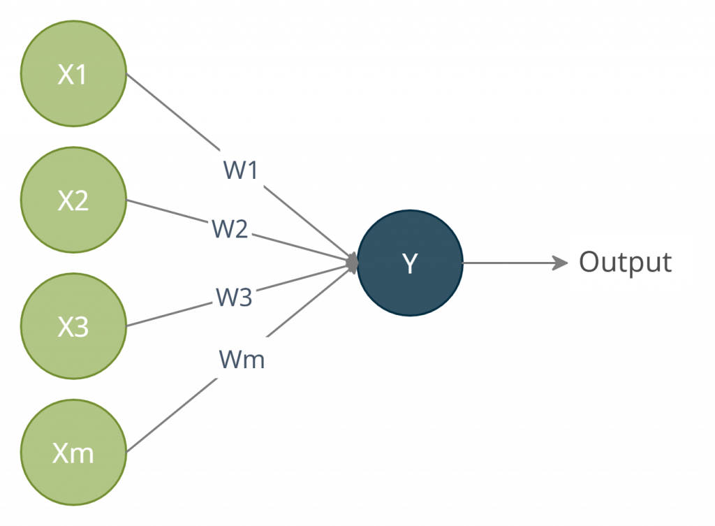
A perceptron is an artificial neuron. Instead of electrochemical signals, data is represented as numerical values. These input values, normally labeled as X (See Figure 2), are multiplied by weights (W) and then added to represent the input values’ total strength. If this weighted sum exceeds the threshold, the perceptron will trigger, sending a signal.

You can call a perceptron a single-layer neural network.

Standard Equation

Equation 1 shows the mathematical characterization of the output Y of a perceptron. If the summation of all weighted values is less than the threshold constant, y equals zero. Otherwise, y equals one.

We can simplify the equation further with Equation 2. This form also makes it easier to code. If the product of wx is greater than b (bias), y will be positive and is therefore True. If the product is less than b, y will be negative and thus False. Note that bias or b is currently the most used notation for thresholds in neural networks.

To demonstrate all these theories, we will create a sample perceptron model that distinguishes whether a dish is cooked good or bad. Let’s call this model – the Gordon Ramsay.

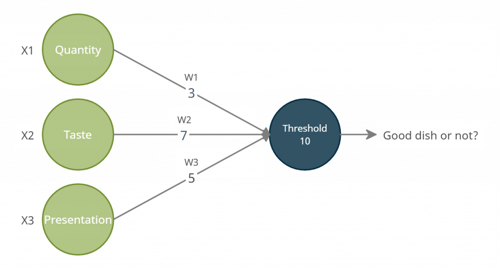
Gordon Ramsay has 3 input criteria: quantity, taste, and presentation. If there are too few or too much of the dish, the quantity criterion returns zero. Similarly, the other criteria return zero if the taste or the presentation is bad.

Quantity	Taste	Presentation	Weighted Sum	Threshold	Good or Bad?
Few (0)	Good (1)	Good (1)	3*0 + 7*1 + 5*1 = 12	10	Good
Enough (1)	Good (1)	Good (1)	3*1 + 7*1 + 5*1 = 15	10	Good
Too Much (0)	Bad (0)	Good (1)	3*0 + 7*0 + 5*1 = 5	10	Bad

To get the weighted sum, Ramsay adds all the products of each criterion’s weights and inputs. Then, it checks if the weighted sum exceeds the threshold constant. If it does, the dish is good. If it is doesn’t, the dish is bad.

But, what if the input values are not binary? This is where other activation functions come in.

Introduction to Activation Functions

Activation functions (aka Transfer Functions) decide whether a perceptron will “activate” or not. It also normalizes the output to a range between 1 and 0 or between -1 and 1. In our earlier example, we used an activation function called a binary step function to represent the standard equation of a basic perceptron.

The problem with the step function is that it only allows 2 outputs: 1 and 0. An input barely above the threshold will have the same value of 1 as an input 10000 times greater than the threshold. High sensitivity can be problematic in learning the weights and bias parameters as even minor changes in the parameters completely flip out the output (Don’t worry if this part does not make sense. This topic will be explained in the next title of our neural network series) To solve this, we can use other activation functions like sigmoid. Unlike the step function, the sigmoid function has an S-shaped curve bound between 0 and 1 (See Figure 5). This makes the gradient smoother, allowing floating outputs for precision.

There are more activation functions in neural networks and deep learning. Each has its own advantages and disadvantages. You will learn them as we proceed with the series. What’s important is you’re gaining intuition on how a single artificial neuron in a neural network works.

That said, we now create a Python Perceptron.

Creating a Perceptron Model in Python

For starters, choose a code editor. I recommend using an interactive shell so you can see the output immediately after entering the code. This way, you can check every variable and output before you perform time-consuming tasks such as training.

Jupyter Notebook is preferred. It’s a combination of a traditional editor and an interactive shell. You can use it to code, see the results, and save. You can even use it as a data visualization tool.

from sklearn.datasets import load_iris
iris = load_iris()
x = iris.data[:,(2,3)]

First, import your dataset from Scikit-learn. Scikit-learn is an open-source machine learning library. It provides various tools for model fitting, data preprocessing, model selection and evaluation, and many other utilities.

Scikit has a package called sklearn.datasets that contains sample datasets for quick testing. Inside this package is the Iris dataset. This data set contains 3 classes of 50 instances each, where each class refers to a type of Iris plant: Iris-Setosa, Iris-Versicolour, and Iris-Virginica. Each instance contains four attributes: sepal length, sepal width, petal length, and petal width.

We will train our model using only petal length and petal width. Moreover, since a perceptron is limited to binary output, our perceptron will only detect whether the Iris plant is an Iris-Setosa or not.

You can see the contents of x in Figure 6. We sliced the array containing the four attributes to obtain the petal width and length details only.

iris.target

By entering iris.target, you will see the list of all 150 instances of Iris plants labeled with the target values: 0 as Iris-Setosa, 1 as Iris-Versicolour, and 2 as Iris-Virginica (See Figure 7).

y = (iris.target == 0)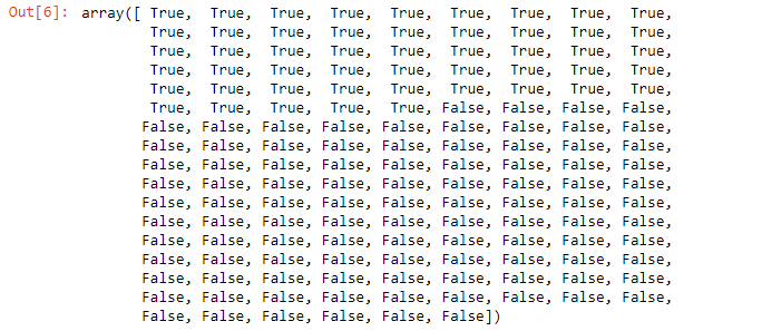

We want the 0-labeled instances since our goal is to detect the Iris-Setosa plant (See Figure 8).

y = (iris.target == 0).astype(int)

Furthermore, we convert the Boolean information into binary integers (See Figure 9).

Now that we have both x and y values, we can now train the perceptron. Import Perceptron from the sklearn.linear_model package.

from sklearn.linear_model import Perceptron

Initialize the parameters with random values, then fit the 150 pairs of petal width and length instances to y. This will teach the perceptron to distinguish the Iris Setosa among the 150 instances.

per_clf = Perceptron(random_state=42)
per_clf.fit(x,y)

Finally, use predict to check if the model works. Enter 2 floating values as hypothetical petal width and length. I used the first value from Figure 6 to confirm the validity of the model. Then, a wise guess for the second value.

ypredict = per_clf.predict([[1.4,0.2],[1.37,0.29]])

Remember!

• A biological neuron only activates if the total input signal exceeds a certain threshold.
• A perceptron is an artificial neuron. It is also a single-layer neural network.
• Activation functions decide whether a perceptron will trigger or not.

That’s it for Perceptrons! See you next time as we move on to Neural Networks.